Ilma is my self-built Navtex decoder for the Raspberry Pi. I sailed 2,000 nautical miles from the Netherlands to Finland and back. Ilma logged every Navtex message on the way.
Reception in the Baltic was disappointing. Whereas in the North Sea Ilma had received daily bulletins, in the Baltic Navtex messages came in only near Gislövshammar and nowhere further north in Sweden or Finland. Ilma’s reception radius was only about 70 nm in the Baltic, against a nominal 300 nm.1
On the return leg, almost at the point where my journey had started, I remembered that I had bought an external Bias-T to power the active antenna – but did not have the time to install it before casting off. When I finally did, reception changed dramatically.
Receiving Navtex in the North Sea vs. the Baltic
My sailing journey led from the Netherlands to Finland via Germany, Denmark and Sweden. Along the track, I measured the quality of reception and decoding in relation to distance from the transmitter station.
Reception faded with distance, as expected, but much faster in the Baltic than in the North Sea. Grimeton and Tallinn were within nominal range for weeks, and neither produced a single station letter. The only trace of Tallinn came from a separate narrowband search2, which found its carrier at 101 and 119 nm while the decoder made nothing of it.
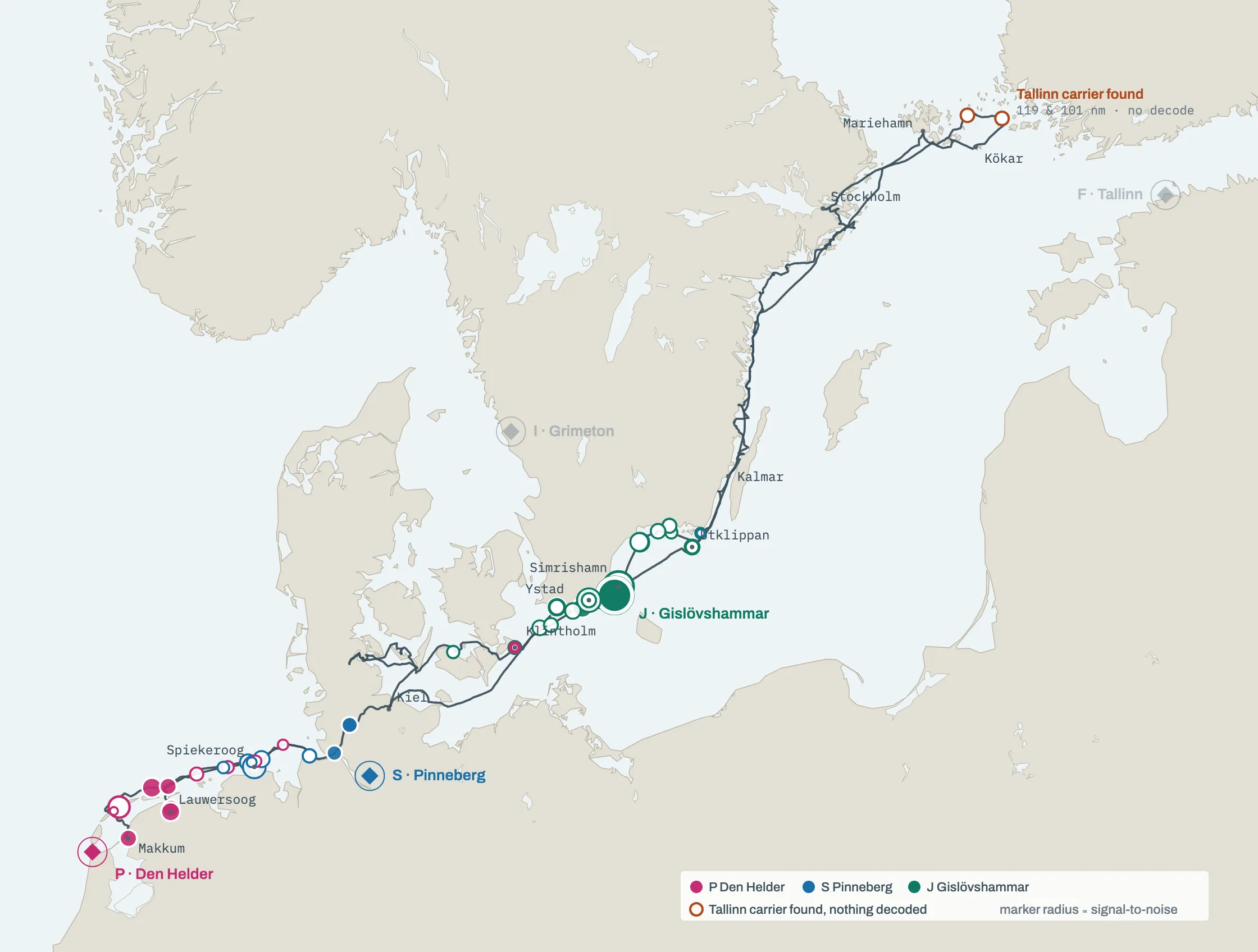
North and east of Stockholm there is nothing. Grimeton and Tallinn are shown because both were within nominal range for weeks without ever decoding a station letter.
The two orange rings off the Turku archipelago are where a narrowband search did find Tallinn's carrier, at 119 and 101 nm, with the decoder making nothing of it.
Measured against its nominal range, Gislövshammar fell about 7.6 dB short.3 About 2.9 dB of that is the sea path itself: the Baltic sea-path penalty.4 The likely reason is under the keel. Groundwave at 518 kHz travels on the conductivity of the surface it crosses,5 and Baltic surface water is brackish, around 6 practical salinity units in the Åland Sea against the North Sea’s 32.6 Any receiver on that path pays the penalty. The remaining 4.7 dB belong to the receiving chain – and that part was my problem.
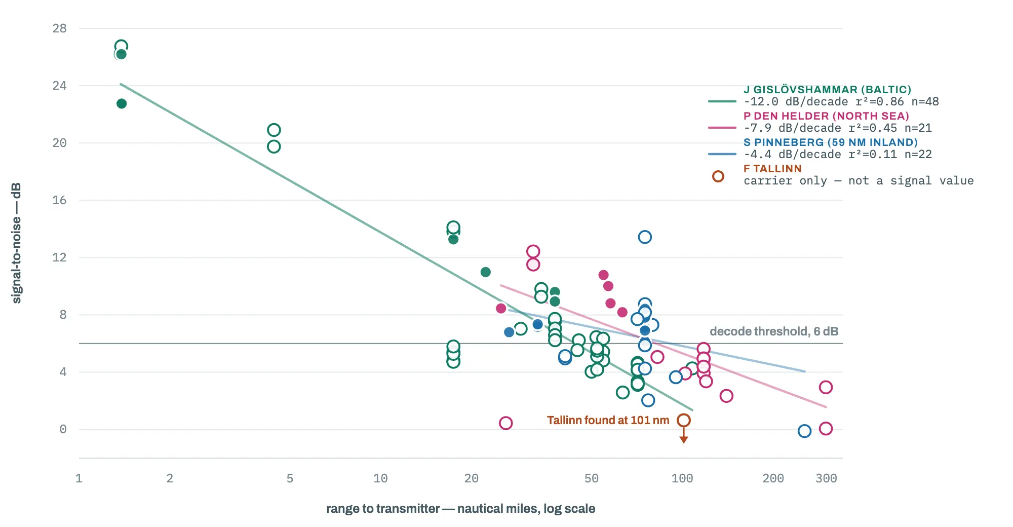
Gislövshammar, over Baltic water, falls at 12 dB per decade of distance; Den Helder, over the North Sea, at 7.9. Pinneberg barely falls at all, because it sits 59 nm up the Elbe from its mouth: what lies in the path matters more than how far away it is.
The orange marker is the Tallinn carrier, found by a different measurement where this one reads nothing, and it belongs to no fit.
Everything but the radio
When no Navtex messages came in anymore, I looked for the cause. I tried to eliminate local noise, I removed other devices, I added more ferrites, and I ruled out tuner gain.
Working on marginal reception forced me to make all kinds of improvements to the code, and reception profited from them. They were mostly about framing and error correction rather than the radio:
- The forward error correction gave up on finding its parity while still inside the phasing preamble, where by construction it could never find it, and fell back to emitting every codeword twice. Fixing that turned one live slot from zero framed messages out of eleven into twelve out of sixteen.
- Carriage returns were spending the shift-state budget and clipping a digit off every wrapped coordinate.
- A bit-phase that slipped across a ZCZC marker cost the framing of the message behind it.
- For recordings, a consensus pass over ten sub-symbol offsets turned 32 erasures into none across three captures.
The most humbling find came last. In August I switched on soft-decision decoding and measured the character error rate falling from 13.0 to 5.8 per cent. Three weeks later I found that the setting had never reached the decoder: every production path sliced the bits to ones and zeros before the magnitudes could be used. The improvement had only ever been true of the test harness.
None of it closed the 4.7 dB gap in the receiving chain. What on earth could I do to close it?
If the complicated explanations fail, it’s the easy one
On an evening on the way back, finally, I looked at the voltage supplied to the active NASA Marine H-Vector antenna: it was lower than it should be. Three months ago, before leaving, I had been glad that the RTL-SDR could supply Bias-T voltage at all and did not want to add another component to the Raspberry Pi setup. Simplicity won, which turned out to be expensive: the dongle provides 4.5 V.7 The antenna’s own specification gives no voltage at all, but the power adaptor NASA Marine sell for running the antenna into a third-party receiver provides 12 V.8 That adaptor was out of stock when I ordered the antenna, so I bought a generic module instead, on AliExpress. Underway, I forgot about the matter, and it was only at the end of the journey that I remembered.
I installed the generic Bias-T module with a 50 kHz to 500 MHz passband. The first reception was disappointing: no signal at all. Ilma writes a telemetry row for every broadcast slot, whether or not anything decodes. That is what showed the dead Bias-T within minutes rather than overnight, and it is what measured the improvement once the repair worked.
I measured the Bias-T module with the multimeter – no power supplied at all. Measuring the internals revealed an open circuit between the fuse and the choke. It was a manufacturing fault. I soldered a bypass.
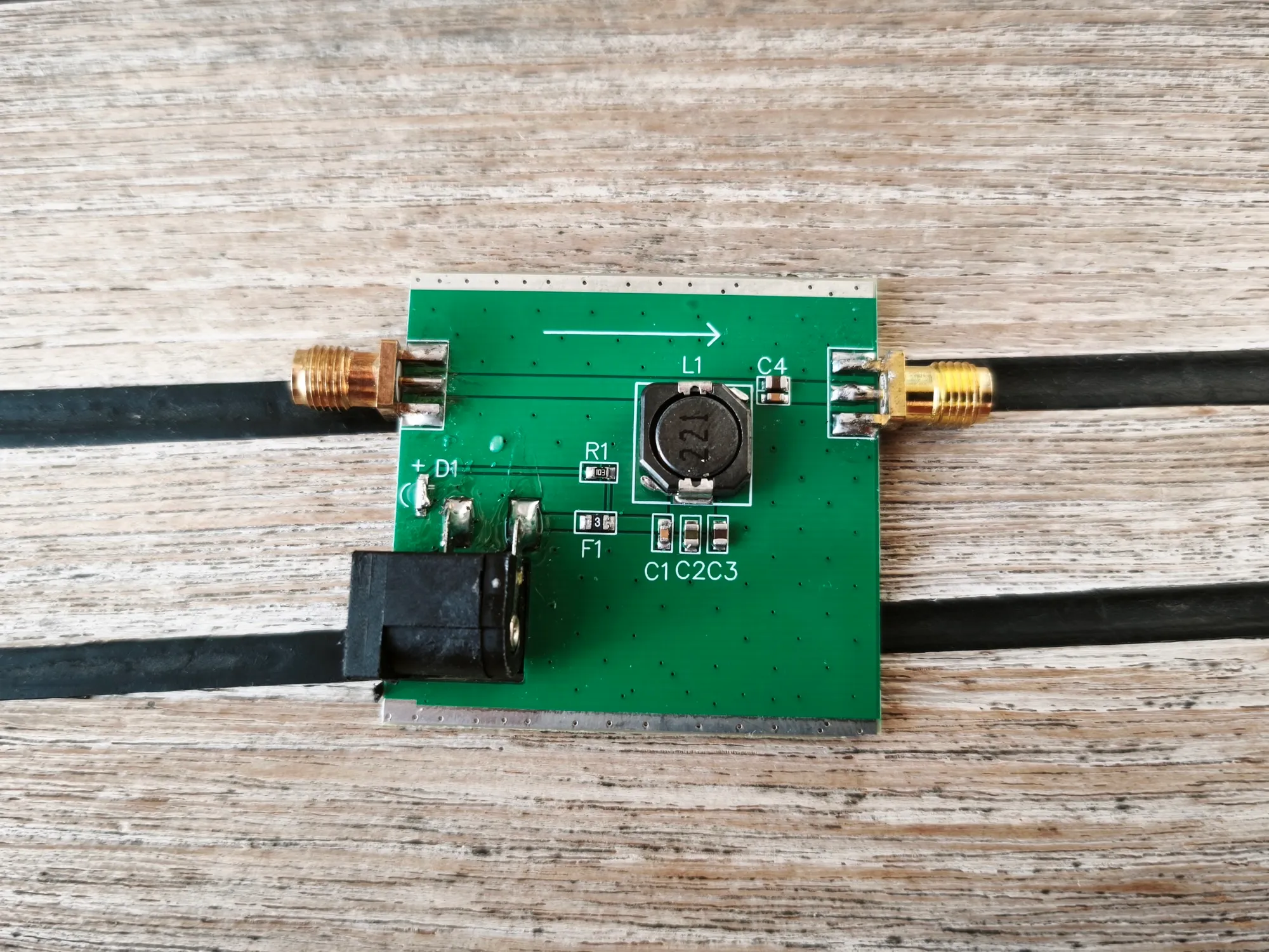
The LED D1 sits across the input, upstream of the break, which is why it glowed the whole time.
Reception with a correctly powered antenna
After supplying 12 V to the antenna, signal-to-noise improved by about 6 dB.9 On the 14:30 UTC pair the signal rose by 12.7 dB and the noise floor by 5.4; the 7.3 dB between them comes down to about 6 once the shorter distance from Sneek and the other slots are taken into account. That is what a preamplifier coming out of starvation does: the gain that lifts the station also lifts the band it sits in. Only the gap between them decodes.
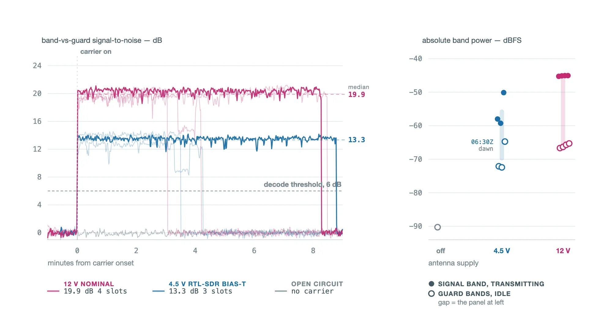
Right: the same recordings as absolute levels. Both the signal and the noise floor rise with supply voltage; what changes is the gap between them, which is the panel on the left. The open-circuit recording sits 18 dB lower again, with no preamplifier gain at all.
The 06:30 UTC slot carries more atmospheric noise than the others because it is a dawn slot, not because of the supply.
The first Navtex message to arrive with the H-Vector on its nominal supply came in framed and legible from end to end: a Den Helder weather forecast, 1830 characters, not one of them flagged as an erasure.10 It begins:
PE57
131104 UTC SEP 26
FORECAST DUTCH EEZ ISSUED AT 11:04 UTC 130926.

GALE WARNINGS.
THAMES. HUMBER. GERMAN BIGHT. DOGGER.
NO WARNING.

SYNOPSIS.
RIDGE OVER THE EAST PART OF ENGLAND WILL MOVE TO DENMARK. WEAK TROUGH IS ALMOST STATIONARY OVER THAMES ON SUNDAY AND WILL MOVE TO HUMBER AND DOGGER ON MONDAY.
…
Also, for the first time, Navtex messages from Oostende came in, in Enkhuizen, at a distance of about 125 nm.
What made this take a whole summer is that every step failed silently: no specification to violate, no error message, a lit indicator on a dead module, and a receiver that kept decoding well enough in the North Sea to look healthy.
The 12 V fix would probably have transformed my southern Baltic reception. But it would not have given me Tallinn from the Åland or Turku archipelago. Between there and Tallinn the signal crosses thousands of granite islands, and a groundwave loses far more over rock than over water. No supply voltage changes the geography.
Footnotes
-
“Reception radius” here is the furthest 20 nm window in which at least half of the scheduled daylight broadcasts still produced a decoded message. Daylight only, because Gislövshammar’s decode rate runs 18 per cent at 01:30 UTC against 38 per cent at 17:30, which reflects the time of day rather than range. The 300 nm figure is the nominal range published for the station in the ITU Navtex station table. The two numbers are not measured the same way and the comparison is indicative, not a like-for-like shortfall. ↩
-
Integrating a 6 Hz slice at the mark and space tones over minutes, scored against neighbouring reference bands, and comparing an on-air window with an off-air control. On 5 August the mark tone rose 0.49 dB above control in 12 of 13 consecutive 20-second windows. The lift is smaller than the control’s own standard deviation, so the detection rests on the sign test rather than on the effect size. A run pointed at Gislövshammar the same evening came back negative, which is the reassuring part. ↩
-
Gislövshammar’s measured range falls 7.6 dB short of its nominal range when converted at the fitted slope of 12 dB per decade. Subtracting the 2.9 dB Baltic penalty, which any receiver on that path pays, leaves about 4.7 dB belonging to the receiving chain. ↩
-
Signal-to-noise regressed on the logarithm of range with a Baltic indicator, across 69 broadcast slots from the two coastal stations, Gislövshammar and Den Helder. Pinneberg was excluded because it sits inland and follows no range law. The Baltic term is −2.88 dB with a standard error of 0.79. Slots recorded at the same berth on the same evening are not independent observations, so that standard error is optimistic. ↩
-
Attenuation of a groundwave is set by the conductivity and permittivity of the surface it travels over. ITU-R Recommendation P.368-10, Ground-wave propagation prediction method for frequencies between 10 kHz and 30 MHz (08/2022), gives the reference curves, with separate cases for sea water of average salinity at 5 S/m and of low salinity at 1 S/m, against 10⁻³ to 10⁻² S/m for dry land. Those curves are computed for fixed values and not for a salinity gradient, so the Baltic penalty measured here is not read off that document. It only says which way the effect has to run. ↩
-
Åland Sea surface salinity of 5.25–6.25 g/kg is from Lehmann et al., Salinity dynamics of the Baltic Sea, Earth System Dynamics 2022;13:373–392. For the North Sea the BSH gives 15–25 PSU where riverine input is high and “32 to > 35 PSU” in the open sea; 32 is the low end of that range, which is the right end for the shallow southern paths these messages crossed. Practical salinity units and g/kg are not the same quantity, but they are close enough to compare at this precision. ↩
-
The RTL-SDR V4’s Bias-T provides 4.5 V at 180 mA, software switchable (datasheet, page 1). This was noted when the receiver was first built, in the hardware section of Ilma, a Navtex Decoder for the Raspberry Pi, without it being appreciated that the active antenna wanted almost three times that. ↩
-
The H-Vector’s own specification states no supply voltage. NASA Marine sell an HF antenna power adaptor for this exact case, described as: “If you want to use the antenna for another receiver you will need this power adaptor to provide 12V.” The figure is therefore inferred from the manufacturer’s own accessory rather than read off a datasheet, which is part of why it went unnoticed for so long. ↩
-
Band-versus-guard signal-to-noise, re-measured from the saved recordings through the decoder’s own measurement. On 12 V: four Den Helder slots at Sneek, 14:30 and 22:30 UTC on 13 September and 02:30 and 06:30 on the 14th. On 4.5 V: three slots at a berth in Leeuwarden, 14:30 and 18:30 UTC on 12 September and 06:30 on the 13th. Sneek is 7.9 nm closer to Den Helder, worth about 0.7 dB at the fitted slope for that station, which is subtracted. The per-slot peak is the largest of some six thousand measurements and moves by up to 1.1 dB when the measurement grid is shifted by a fraction of one window; the 99th and 95th percentiles and the median across the transmission move by less than 0.1 dB. All four statistics put the improvement between 5.8 and 6.0 dB. A recording from the Leeuwarden berth while the Bias-T was broken reads 3.94 dB and serves as the zero. The absolute levels in Figure 4 are the signal band while transmitting and the guard bands while idle, measured the same way. ↩
-
Den Helder P, message E57 of 13 September, received 14:34 UTC at Sneek. 1830 characters, framed, with the station and serial read correctly and no erasure markers in the body. It is not literally perfect: one sentence reads “A LIGHT HOWER” where the three parallel sentences around it read “A LIGHT SHOWER”, so one character was lost without the decoder noticing. That is one substitution in 1830, against a run of half-readable slots before it. ↩