04/09/2026

Dead Reckoning

A sailing film needs to tell the viewer where the boat is. Sailors record their voyages as GPS tracks – recorded by a tablet or smartphone running Navionics, or a chartplotter. How to create a visually attractive representation of these tracks?

The usual ways of doing it are a screen recording of the chart plotter or a Google Earth flyover, and both look like what they are. My Python script gpx_overlay.py takes a different route. It reads GPX tracks – exported from Navionics, Orca or a chartplotter – and writes two PNG layers of identical size: a basemap of coastlines, and a track with a transparent background. The sea can be left fully transparent, so the layers drop into Final Cut over the footage and the water underneath is the actual water the boat sailed through.
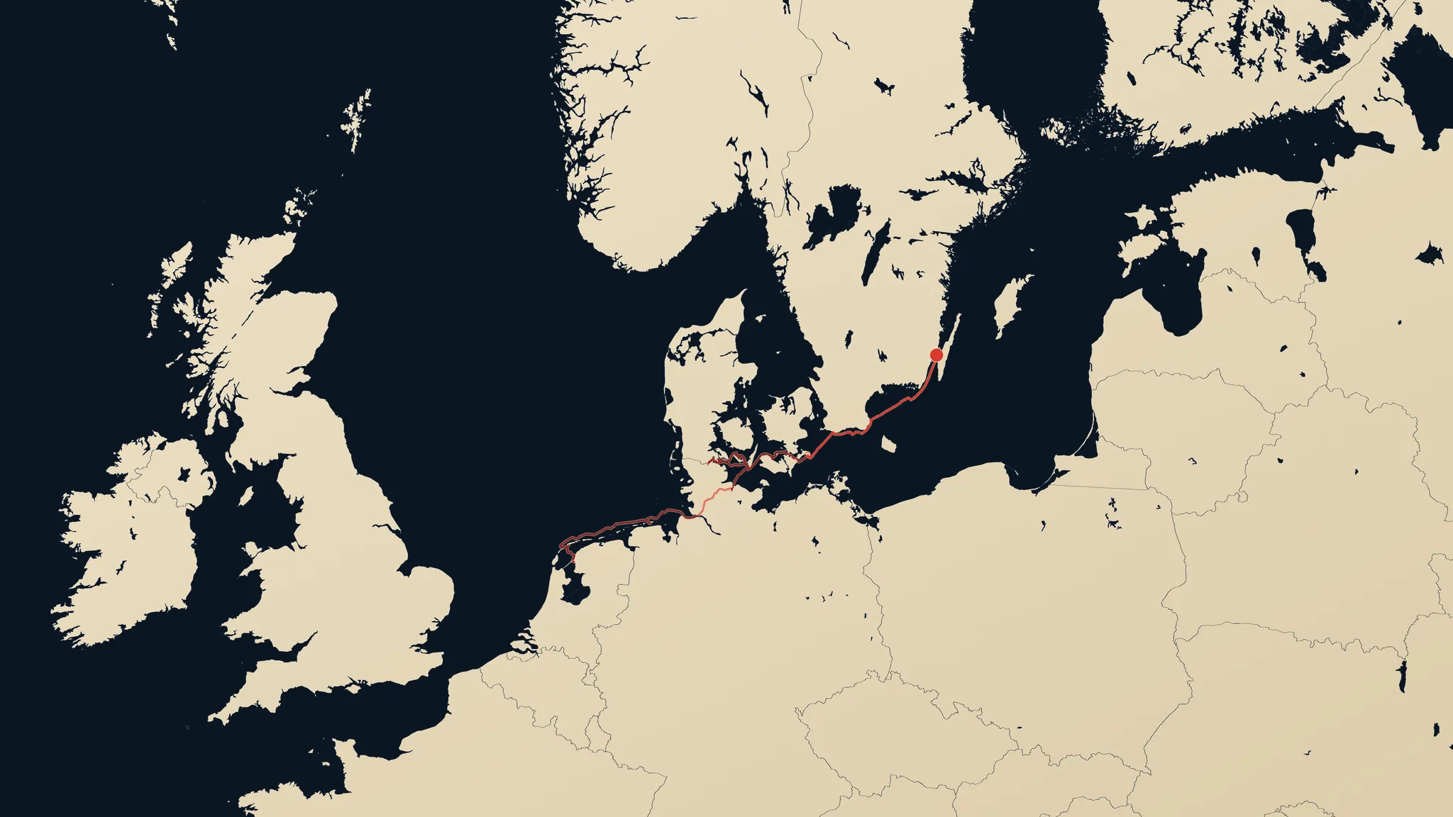
A position card in the parchment style: warm paper land, a navy hairline along every coast, and the passage from the Frisian islands to the Baltic drawn in red, ending at a dot off Kalmar.

Figure 1. One card from the set, at the shared frame that holds across all of them. The sea in the file is fully transparent and is shown here over flat navy; in the edit, footage runs underneath it. Earlier legs are drawn at reduced opacity, the current leg at full weight, and the dot marks the position the card is cut to.

The script is 661 lines of Python with two dependencies, NumPy and Pillow, plus ffmpeg if a ProRes file is wanted at the end. What follows are the parts that were not obvious before writing it.

The tracks have no clock

Not every GPX file has a clock in it. Phone apps generally stamp every point with a time, but Raymarine plotters export without <time> elements at all: the file records where the boat went and says nothing about when. Where that is the case it rules out the obvious animation, which is playback against elapsed time, and it rules out any derived speed. The script therefore never reads a timestamp, so the same code path serves both kinds of file.

The substitute is distance. The script accumulates great-circle distance along the track and uses that as the time axis:

def cumulative(lines):
    """Per-polyline cumulative distance along the whole run, and the total."""
    cums, total = [], 0.0
    for pts in lines:
        c = [total]
        for i in range(1, len(pts)):
            total += haversine(pts[i - 1], pts[i])
            c.append(total)
        cums.append(c)
    return cums, total

Every position query then becomes a lookup by distance rather than by time. point_at() binary-searches the cumulative array and interpolates linearly between the two bracketing vertices, and slice_between(d0, d1) returns the stretch of track covered between two distances, cutting partial segments at both ends.

The consequence is that the boat draws at constant speed over the ground. A tack-heavy beat and a broad reach take screen time in proportion to the miles sailed, not the hours spent. Two nights at anchor take no screen time at all, because the plotter logged no distance. The animation is flattering, and it is honest about geometry rather than about the passage.

This is also why the mid-voyage position cards work the way they do. --end-at LON,LAT does not cut the track at a coordinate; it finds the track vertex nearest that coordinate and cuts there, then reports how far off the request was:

cut at 9.5797 E 54.8977 N, 0.67 nm from the point asked for

That number matters. It tells the editor whether the card shows the place they asked for or the nearest place the boat actually passed.

The map has to share the track’s projection

The script holds one projection function, spherical Mercator in metres:

def mercator(lonlat):
    v = np.asarray(lonlat, dtype=float).reshape(-1, 2)
    lat = np.clip(np.radians(v[:, 1]), -1.4835, 1.4835)
    return np.column_stack([
        np.radians(v[:, 0]) * EARTH_R,
        -EARTH_R * np.log(np.tan(np.pi / 4 + lat / 2)),
    ])

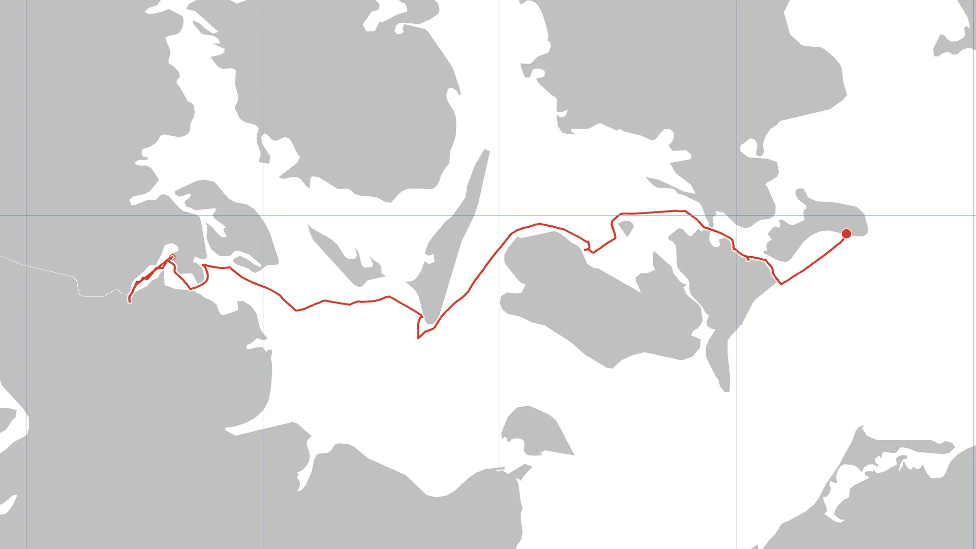
Coastlines come from Natural Earth 10 m vector data1 and pass through that same function, with the same scale and offset, before anything is drawn. Alignment is not measured or corrected. It is exact by construction, because a coastline vertex and a track vertex at the same coordinate cannot land on different pixels when one function maps both.

--verify is the check on that claim. It flattens map and track into one image and rules a graticule over both at one degree, in the same projection:

The Flensburg to Klintholm leg over a plain grey basemap with a one degree graticule ruled over it. The track threads the channels between the Danish islands and stays off the land.

Figure 2. The alignment check, in the plain style rather than the parchment one because it is an instrument, not a picture. The evidence is negative, and it is the only evidence that counts here: the track threads the gaps between the Danish islands and never once crosses a coastline. Several of those gaps are narrower than a mile, so a basemap off by a mile would beach the boat somewhere in this frame. The graticule comes from the same `mercator()` call as everything else, which is why it can be trusted as a ruler rather than a decoration.

Framing is derived once, from the projected extent of the track, padded and then stretched on one axis to match the output aspect ratio:

if w / h < aspect:
    g = (h * aspect - w) / 2
    x0, x1 = x0 - g, x1 + g

--bounds W,S,E,N overrides that with an explicit window, which is what holds one frame across a whole set of cards so they cut together without a jump.

Feature rejection is a bounding-box test in degrees, not in pixels. lonlat_window() inverts the four corners of the output box back to longitude and latitude, and any polygon whose bounding box misses that window is skipped before it is projected. Drawing the Baltic therefore does not pay for the Pacific.

Ink is what makes it read as a chart

The basemap is built as a mask first. Land polygons and minor islands are filled white, interior rings and lakes are punched back out to black, and that single mask drives everything else:

for ext, holes in land:
    md.polygon(ext, fill=255)
    for h in holes:
        md.polygon(h, fill=0)

The parchment style then fills land with a paper gradient and leaves the sea fully transparent. That combination has a problem: with no colour difference between land and sea, and no sea at all, there is nothing to define a coast. A hairline stroked around every ring solves it. The stroke is drawn for lakes as well as land, and it survives where land meets land, which a fill boundary does not.

The drop shadow is cast by the land mask, blurred, offset, and composited under the land rather than over it. Because the land is opaque and the sea is not, the shadow only ever falls seaward, which is what keeps a coastline legible when moving footage shows through underneath.

The paper gradient is computed at 64 by 64 and resized bicubically to the output size. A diagonal wash has no high-frequency content, so the small array loses nothing and the large one would cost a second per card for no visible gain.

Two pixel problems worth knowing

Pillow’s ImageDraw writes pixels, it does not composite them. A stroke laid over an earlier stroke replaces it, alpha included. The track is drawn with a light halo underneath it for legibility over dark footage, and drawing halo and line onto the same surface means each frame’s halo bites a notch out of the previous frame’s line end. The halo therefore lives on its own RGBA layer and the two are alpha-composited only at the point a frame is written.

Redrawing the whole track every frame is quadratic. The animation instead keeps a persistent line layer and adds only the stretch newly covered since the last frame:

def advance(target):
    nonlocal drawn_upto
    if target <= drawn_upto:
        return
    new = [px(seg) for seg in slice_between(live_lines, cums, drawn_upto, target)]
    if halo:
        draw_lines(hd, new, halo, hw)
    draw_lines(ld, new, colour, lw)
    drawn_upto = target

Antialiasing is supersampling: everything is drawn at three times the output size and reduced with a Lanczos filter at the end. This is the script’s memory ceiling. A 3840-pixel card at --ss 3 draws into 11520 by 6480, three persistent RGBA layers of it plus the composites, and that is the practical reason not to raise the default.

Determinism, because cards have to match

Cards rendered days apart have to be interchangeable on the timeline. Three things enforce that. The paper grain uses a fixed seed, np.random.default_rng(7), so repeat renders are byte-identical rather than merely similar. --bounds pins the frame independently of which track is being drawn. --reuse-map skips the basemap entirely if a correctly sized one is already in the output directory.

The guarantee holds in practice. A card added to the set a day later, with the earlier renders no longer on disk and the basemap therefore redrawn from scratch, differed from the reference card in 0.121 per cent of pixels, all of them inside the route’s bounding box. The land was pixel-identical.

Output

Three modes. --verify writes the flattened alignment check of Figure 2. --still writes one finished frame with alpha, plus a flattened preview. The default writes a numbered PNG sequence, optionally encoded to ProRes 4444 with a real alpha channel:2

ffmpeg -c:v prores_ks -profile:v 4444 -pix_fmt yuva444p10le -alpha_bits 16

What it does not do

The projection is spherical Mercator only, which is fine for the usual cruising areas and would be a poor choice above about 70 degrees north. The animation cannot show time if the data is not available, so it cannot show a night at anchor, a gale spent hove to, or any speed at all. And the styling is a fixed pair of presets with per-flag overrides rather than anything data-driven, which is enough for one film series and would not be enough for a second one in a different register.

None of the machinery above is sailing-specific, though: only the two styling presets are. The parser, the distance clock, the projection and the drawing pipeline never learn what produced the track, so a hiking, cycling or driving log from a handheld receiver or a phone goes through the same code path as a passage. Inland it is the basemap that would want work, because Natural Earth carries coastlines, lakes and borders but no roads. Point the loader at a vector source that has them, and the script would draw a drive across Europe or a walk across a country as readily as it draws a crossing of the Baltic.

Footnotes

  1. Natural Earth 10 m physical and cultural vectors, fetched as GeoJSON from martynafford/natural-earth-geojson and cached beside the script on first use.

  2. ProRes 4444 is the codec to use here rather than 422, which has no alpha channel at all. -alpha_bits 16 keeps the matte from banding at soft edges.